Statistical Modeling : Simple Linear Regression

Statistical Modeling

Statistical modeling is the practice of summarizing observation and create inferences from it. observation represented in data points includes lots of details. for example, if we observe house sales information in a certain location, we could collect information on the size of the house, price, location, etc.. for now let’s assume that we are concerned only with price and square footage of the house. we observed 100 house sales. there is going to be a lot of information in this data set that we don’t necessarily want to keep track of. imagine now we have 1000 observations (data points). Statistical modeling enables us to create summaries from data, to describe the general trend or overall shape of the data without keeping all track of all observation and data points. Statisticians sometimes refer to this idea by data compress.

%matplotlib inline
import matplotlib as mpl
import matplotlib.pyplot as plt
mpl.rc('axes', labelsize=14)
mpl.rc('xtick', labelsize=12)
mpl.rc('ytick', labelsize=12)

import numpy as np
np.random.seed(56)
X = 2 * np.random.rand(100,1)
y = 8 + 5 * X  + np.random.randn(100 ,1)

plt.plot(X,y, "b.")
plt.xlabel("X", fontsize=12)
plt.ylabel("y", rotation=0,fontsize=12)
plt.show()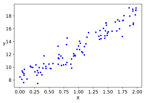

The first task of statistical modeling is to summarize or compress this information through a representative model describing correlations in the data. but it does not stop there. Modeling enables us to enter the realm of inference - if we are trying to extend our knowledge from the data we have already, to other variables we have not to measure or didn’t measure directly - essentially extrapolating from sample data to a larger population is an inference based on modeling.

But more importantly, observations are prone to measurement errors, whether this has to do with mistakes, deliberate lies, possibly incorrect assumptions made at various stages, accidents,etc.. some of these sources for error are systematic where it will distort data in predictable, repeatable ways. but some other sources of errors are statistical it is directionless, do not repeat itself yet the distribution of errors in data is still predictable and stable (probability theory helps us to handle such errors).

Simple Linear Regression Model

The most basic of all statistical models and a foundation of most predictions in the world of machine learning is Simple Linear Regression. The model of two random variables, $y$, and $X$ , where we are trying to predict $y$ from $X$. and like any good statistical model, it has a few key assumptions:

1. $X$ distribution is unspecified, possibly even deterministic.
2. $y \mid X = \beta_0 + \beta_1x + \epsilon$ , where $\epsilon$ is a noise variable.
3. $\epsilon$ has mean 0, a constant variance $\sigma^2$, and is uncorrelated with $X$ and uncorrelated across observations.

the model assumes a noise $\epsilon$ normally distributed Gaussian to represent measurement error or fluctuations in $y$, or both. The coefficient $\beta_0$ represents and intercept or initial state. where the coefficient $\beta_1$ represent weights added to variable $X$ to predict $y$.

We could plot a simple regression model on the above dataset to compress and summarize the description of the data.

X_b = np.c_[np.ones((100, 1)), X]
beta_1 = np.linalg.inv(X_b.T.dot(X_b)).dot(X_b.T).dot(y)
X_new_b = np.c_[np.ones((100,1)), X]
y_predict = X_new_b.dot(beta_1)

# Plot model predictions
plt.plot(X, y_predict, "r-")
plt.plot(X, y, "b.")
plt.show()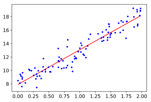

As you can see from the plot, the regression model line compresses the 100 data points into a simpler linear upward trend that is easy for humans to remember and reason about. even better it helps us predict other data points that obey the same assumptions of the simple linear regression model.

Linear Regression probably the most basic simplest and popular tool in regression modeling. dating back to the late 19th century. its basic assumption a linear relationship between input random variable $x$ and target random variable $y$. This linear relationship can is represented by the algebraic formula $y \mid X = \beta_0 + \beta_1x + \epsilon$ . In simple terms, $y$ can be expressed as a weighted sum of the inputs $X$, with additive noise $\epsilon$ to the observations. and as we described earlier the assumption is this noise is well behaved following a Gaussian distribution. In our introductory example, we can describe the price of a house given an input of the area of the house using a linear model as $price = \beta_0 + w_{area} \cdot area$ .

Where:

• $\beta_0$: is bias (sometimes called intercept or offest).
• $w_{area}$: are weights determine the influence of the area on the target (house price)

We can generalize this model for more than one input or feature to describe a linear relationship between inputs to a target variable. for example, we can describe the relationship between house prices with respect to house area and the number of rooms. $price = \beta_0 + w_{area} \cdot area + w_{rooms} \cdot rooms$

The goal in designing a linear model in the machine learning world is to build a model from a training dataset to help us predict future target $y$ values. for example, predicting house prices given area and number of rooms. So if we have an input observations dataset $X$ the goals become to choose weights $w$ and a bias $\beta_0$ such that on average, the predictions made with this model are as close as possible (fit) the true house prices we observed in the data.

The predicted $y$ values is referred to in mathematical notation using the hat symbol $\hat{y}$

$\hat{y} = \beta_0 + w_1 \cdot x_1 + ... + w_d \cdot x_d$ In high dimentionality suitations we collect all input features in a vector $\mathbf{X}$ and all weights into a vactor $\mathbf{w}$. then the model can be expressed concisely using dot product.

$$\hat{y} = \beta_0 + \mathbf{w}^T \mathbf{X}$$

but before we start finding the best parameters $w$ and $\beta_0$ for our model we will need first to have a quality measure for the given model. that is how do we know that our model was able to predict $y$ correctly. and once we can measure model performance we will need a procedure to improve the model’s prediction quality.

Measure of Quality

Measuring the quality of linear model prediction is key to improve model prediction quality. that is we need a measure of fitness before we start fitting the model to data. Loss Function quantify the distance between the real and predicted value of the target variable. The loss will usually be a non-negative number where smaller values are better and perfect predictions incur a loss of $0$.

Sum of Squared Errors

This is the most popular loss function in regression problems. for a data point $i$, and real target $y_i$ and predict value $\hat{y_i}$. the squared erros is given by:

$$l_i(\mathbf{w}, \beta_0) = \frac{1}{2} \left(\hat{y}_i - y_i\right)^2$$

To measure the quality of a model on the entire dataset, we simply average (or equivalently, sum) the losses on the training set.

$$L(\mathbf{w}, \beta_0) =\frac{1}{n}\sum_{i=1}^n l_i(\mathbf{w}, \beta_0) =\frac{1}{n} \sum_{i=1}^n \frac{1}{2}\left(\mathbf{w}^\top \mathbf{x}_i + b - y_i\right)^2$$

When training the model, we want to find parameters ($\mathbf{w}^, \beta_0^$) that minimize the total loss across all training samples:

$$\mathbf{w}^*, \beta_0^* = \operatorname*{argmin}_{\mathbf{w}, \beta_0}\ L(\mathbf{w}, \beta_0).$$

Linear Regression happens to be one of the models that have an analytical solution to the optimization problem. other more complicated models don’t have a solution that can be solved analytically by a simple formula yielding the global optimum; in which case a numerical solution can be used to optimize the model like Gradient Decent algorithm. I’m not going in the mathematical details for how to optimize Linear Regression analytically, we can subsume the bias $\beta_0$ into the weight parameter $w$ and the final formula for computing optimum w would be:

$$\mathbf{w}^* = (\mathbf X^T \mathbf X)^{-1}\mathbf X^T y.$$

you can easily implement the above formula using NumPy to compute the weights for linear regression. but don’t get used to this easy life, mathematical analysis is not always easy to compute.

w = np.linalg.inv(X.T.dot(X)).dot(X.T).dot(y)
print(w)

Gradient Descent to the Rescue!

For high-dimensionality and nonconvex loss surfaces (surfaces with more than single minima), the Gradient Descent algorithm is an effective model in practice to optimize the model. the key idea behind the algorithm is to iteratively reduce the error by updating parameters in the direction that incrementally lowers the loss function. On convex loss surface (Single Global Minima) it will converge to the minima; the same can’t be said for nonconvex surfaces but at least it will lead towards a local minimum.

Real World Example

Let’s try Linear Regression out on a real dataset. Below I’m going to load in a dataset of Seattle housing prices from here It has the following features:

• id: a notation for a house
• date: Date house was sold
• price: Price is the prediction target
• bedrooms: Number of Bedrooms/House
• bathrooms: Number of bathrooms/House
• sqft_living: square footage of the home
• sqft_lot: square footage of the lot
• floors: Total floors (levels) in house
• waterfront: House which has a view to a waterfront
• view: Has been viewed
• condition: How good the condition is ( Overall )
• grade: overall grade given to the housing unit, based on King County grading system
• sqft_above: square footage of house apart from the basement
• sqft_basement: square footage of the basement
• yr_built: Built Year
• yr_renovated: Year when the house was renovated
• zipcode: zip
• lat: Latitude coordinate
• long: Longitude coordinate
• sqft_living15: Living room area in 2015(implies– some renovations) This might or might not have affected the lot size area
• sqft_lot15: lotSize area in 2015(implies– some renovations)

We minimally process the data to make it amenable to analysis as follows:

• fill in any missing data with the average value for that column
• delete the date and the value sqft_basement

We don’t have to reinvent the wheel, so we will use the most common implementation of linear regression, found in sklearn library. sklearn is the standard package used for the majority of (non-neural network based) machine learning techniques. It contains nice implementations with a common interface for the majority of commonly encountered techniques.

from sklearn.linear_model import LinearRegression

# kc_house_data
# https://www.kaggle.com/shivachandel/kc-house-data
# House sales in King County, Washington State


data = pd.read_csv('kc_house_data.csv')
data = data.drop(['date','sqft_basement'],axis = 1)
data = data.fillna(data.mean())

model = LinearRegression()
model.fit(data.drop('price',axis=1),data['price'])
print("R squared of full model is: {}".format(model.score(data.drop('price',axis=1),data['price'])))

Read More:

• Ruelle, David (1991). Chance and Chaos. Princeton, New Jersey: Princeton University Press.
• Smith, Leonard (2007). Chaos: Avery Short Introduction. Oxford: Oxford University Press.